i2MassChroQ User Manual
- Preface
- 1 Generalities
- 2 Fundamentals in Bottom-up Proteomics
- 3 The main program window
- 4 Exploring identification data
- 5 Exploring post-translational modification data
- 6 Advanced Proteomics Configurations
- 7 i2MassChroQ and Quantitative Proteomics
- 8 Specific procedures for the timsTOF line of instruments
- A GNU General Public License version 3
7 i2MassChroQ and Quantitative Proteomics
This chapter describes in detail the way to prepare the work that will be carried over by the MassChroQ module.
7.1 Interface to the MassChroQ Quantitative Proteomics Module #
While it is certainly possible to perform pretty thorough analyses by exploring data by way of peptide identification—protein inference scrutiny strategies, it is necessary to expand the boundaries of these strategies if quantitative proteomics projects are being developed. We have now integrated MassChroQ in i2MassChroQ, which makes it straightforward to perform quantitative proteomics work right after the identification—protein inference process.
The way the MassChroQ program is harnessed in i2MassChroQ is according to the following outline:
Open an i2MassChroQ project or load protein identification results files;
Configure all the aspects of the MassChroQ run in a specific MassChroQ configuration window;
Use i2MassChroQ to run the external MassChroQ software or have i2MassChroQ only write the file that MassChroQ uses to perform its quantitative proteomics task at a later stage and outside of i2MassChroQ.
7.1.1 Preparing sample associations for MassChroQ #
Performing quantitative proteomics experiments most likely involves comparing samples between them. That means that most often multiple samples need to be associated into meaningful groups. Before going on with the MassChroQ configuration, it is thus necessary to first define the sample associations. In fact, since a given sample is actually a given LC-MS run, and that each MS run's data are then used to perform protein identifications, these assocations are performed between MS runs.
To perform a quantitative proteomics experiment, the very first step is to
load either the protein identification results (see Section 3.4, “Loading the Protein Identification Results” or an xpip project file (see Section 3.5, “Loading i2MassChroQ projects”).
Once the protein identification results have been loaded (or the i2MassChroQ project file), the sample associations (that is, between MS run files) need to be performed by first clicking onto the View MS identification list button of the main program window (see Section 3.4.2, “Displaying the MS Identifications List”). The MS runs are displayed in a table and sample associations can be performed by right-clicking onto the cells of the Alignment group column label, as shown in Figure 7.1, “Defining sample associations for XIC alignments”.
Note
The sample (MS run) associations are critical not only because one wants to compare quantitative data about somehow related samples, but also because of the way MassChroQ performs quantification of proteomics data. Indeed, MassChroQ uses not spectral count-based strategies but an area under the curve strategy where the area of mass peaks is determined by looking at XIC chromatograms for these mass peaks. The associations will thus allow the software to perform the alignment of the XIC chromatograms that will be essential for the quantification analysis. Indeed, even LC-MS runs of an identical sample will not provide identical (m/z,retention time) pairs. But, to be able to quantify proteomics data on the basis of the area under the curve of XIC chromatogram peaks, it is necessary that all the XIC chromatograms for all the associated samples be properly aligned.
The associations between samples can be performed in any arbitrary way, according to the user's experimental scheme. Any number of groups can be defined that may contain any number of samples. The process is described in Figure 7.1, “Defining sample associations for XIC alignments” and Figure 7.2, “Sample associations are done by grouping samples into groups”.
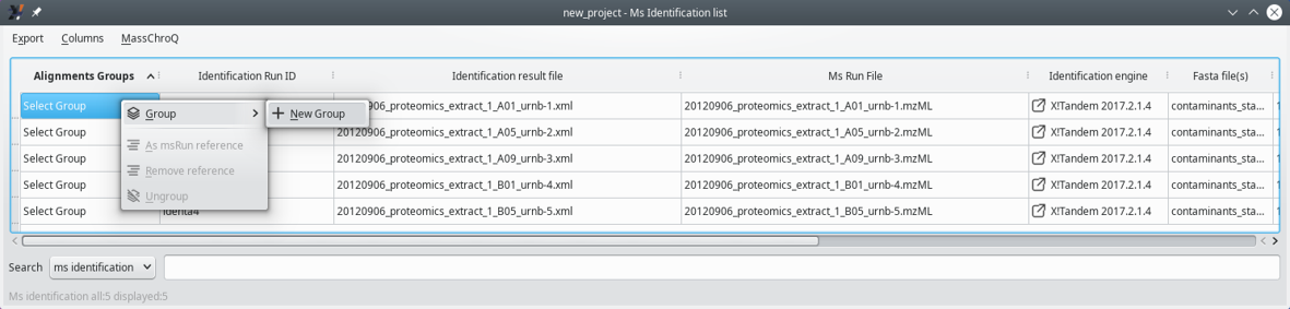
By right-clicking into the cells of the Alignment groups column, groups can be defined and samples can be associated to the groups.
Figure 7.1: Defining sample associations for XIC alignments #
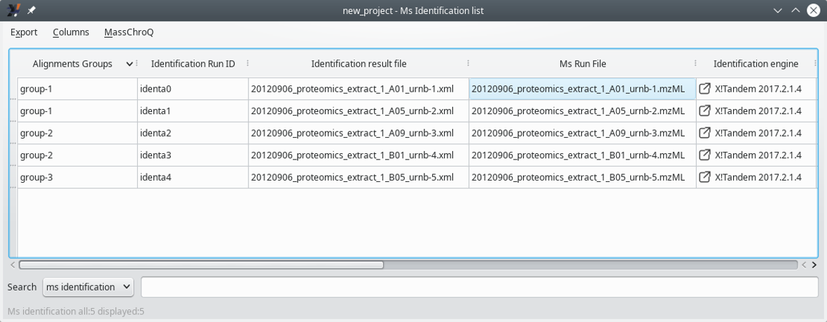
Three groups have been defined, two groups having two samples each and one group having only one sample.
Figure 7.2: Sample associations are done by grouping samples into groups #
Tip: Sample associations with specific sample sets
Sample associations play a critical role when samples (that is, MS runs) have conceptual relationships. For example, let's assume that a project used polyacrylamide gel electrophoresis as a protein separation method. Five related samples (be them biologically-relevant variants or technical replicates, for example) have been loaded onto five different lanes of the gel. The migration pattern between the five lanes is very similar and one could observe reproducible bands (albeit with different intensities) from one lane to the other, say, in sample 1 a band A, below a band B and so on. Sample 2 would also have that pattern, with a band A and a band B, and the same for the remaining samples (that is, lanes). Bands would be excised and subjected to trypsin digestion, the peptides would be extracted and analysed by mass spectrometry. The sample associations, here, would typically involve the definition of groups that associate related “horizontal” bands on the gel. For example, group A would associate all the bands A from the five samples, group B would associate all the bands B from the samples and so on. The sample associations would thus allow the quantification and comparison of kin proteins from the various samples.
The alignement of XIC chromatograms computed for samples from a given association group is performed by having one reference sample in that group. Each group must have a reference sample. The definition of the reference sample can be performed by the user at this stage (or at a later stage, described later) by using the context menu shown in Figure 7.3, “Setting the reference sample for the alignment”.
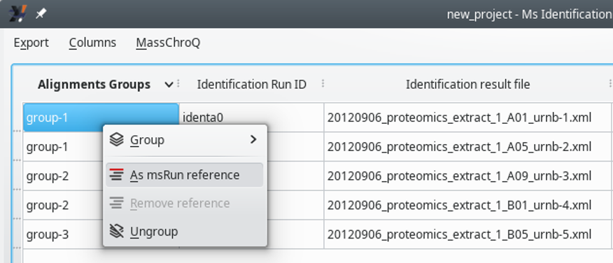
Use the context menu by right-clicking on the cells in the Alignment groups column to set the alignment reference in each group.
Figure 7.3: Setting the reference sample for the alignment #
Note
Selecting the proper alignment reference is not something to do without thinking because the reference sample will serve as the basis for the alignement of all the samples in the group. The best sample to be chosen as alignement reference is the sample that shares the most precursor ions' m/z values with all the other samples. It is possible to delegate to i2MassChroQ the choice of the alignment reference sample, as described later.
Now that the sample associations have been performed, the next step is to configure MassChroQ from within i2MassChroQ. This is described in the next sections.
7.1.2 Configuration of MassChroQ #
i2MassChroQ provides an interface to MassChroQ, the software that performs XIC extractions for a list of precursor ions' m/z values. That interface is shown by selecting the menu item of the main menu. The window that opens up is shown in Figure 7.4, “The MassChroQ interface window (Sample associations)”, and is described below.
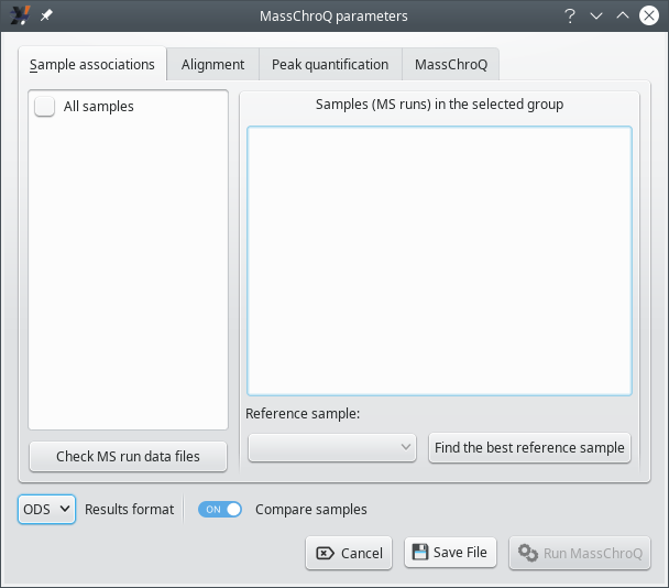
This window offers an interface to the MassChroQ program. The Sample associations tab allows one to define groups of samples that will be processed together. All the configurations in the tabs are described in the sections below.
Figure 7.4: The MassChroQ interface window (Sample associations) #
7.1.2.1 The Sample associations Tab #
This tab allows one to configure the sample associations. The window state shown in Figure 7.4, “The MassChroQ interface window (Sample associations)” corresponds to a situation in which the user did not define sample associations according to the way described in Section 7.1.1, “Preparing sample associations for MassChroQ”. In this case, it is assumed that the user wants to treat all the samples as a single group, (the All_samples group). To reveal all the samples (that is, MS runs) that are being handled, check the All_samples check button, which will associate all the samples in that single group and display them in the right hand side list widget, as shown in Figure 7.5, “The MassChroQ interface window (Sample associations) - all samples listes”.
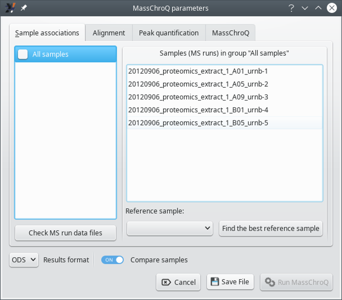
By checking the All_samples check box on the left hand side list widget, all the samples in the project are associated in a single All_samples group and displayed in the list widget on the right hand side of the window.
Figure 7.5: The MassChroQ interface window (Sample associations) - all samples listes #
If the user has crafted groups of associated samples, as described in Section 7.1.1, “Preparing sample associations for MassChroQ”, the window displays different settings at start (see Figure 7.6, “The MassChroQ interface window (Sample associations) - pre-defined sample associations ”).
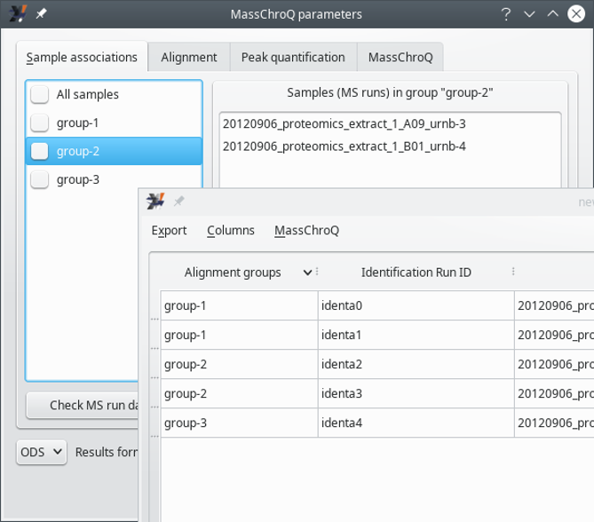
When the sample associations were defined before opening the MassChroQ interface window (the inserted window corresponds to Section 7.1.1, “Preparing sample associations for MassChroQ”), the groups of associated samples are displayed in the list widget on the left hand side of the window. Selecting group names in that list allows one to display the samples associated in a given group. To include a group in the MassChroQ computations, check the corresponding check box widget.
Figure 7.6: The MassChroQ interface window (Sample associations) - pre-defined sample associations #
To verify which samples are being associated in a given group, select that group in the list widget on the left hand side of the window.
To make sure a given group is going to be accounted for by i2MassChroQ during the preparation of the file that lists all the precursor ions' peaks for which the XIC extractions needs to be performed at a later stage by MassChroQ, check the corresponding check box.
The Check MS run data files button allows the user
to make sure that all the samples associated in the various groups can
be found as mass spectrometry data files (mzML or mzXML files). This is a hard requirement
because MassChroQ does the quantification of peptide mass spectrometric
signals by extracting ion current for the peptide's precursor ion (XIC
extraction). For this to be possible, the software needs to access the
mass spectrometry data files.
The Reference sample drop-down list widget allows one to select the alignment reference sample for the currently selected sample association group in the left hand side list. The alignment reference sample must be chosen with care, as explained in Figure 7.3, “Setting the reference sample for the alignment”.
Tip
If the selection of an alignment reference sample is not possible, the user might ask i2MassChroQ to search for it by clicking the Find the best reference sample button. i2MassChroQ will look into all the sample files associated in the current group and search for the sample that shares the maximum number of precursor ions with all the other samples. The discovered MS run file is then set to the drop-down list widget.
The Results format drop-down list widget allows the user to select the kind of format that the quantification results should be written in. The ODS format is the standard format for the LibreOffice software suite. The TSV format is a “tab-separated values” text format.
The Compare samples switch indicates if the results output file should display a low-details version of the data but arranged in a manner that allows the user to easily compare the quantification data about the various samples.
7.1.2.2 The Alignment Tab #
This tab allows one to configure the way the XIC chromatograms obtained for the different associated samples are aligned (see Section 7.1.1, “Preparing sample associations for MassChroQ”) as shown in Figure 7.7, “The MassChroQ interface window (Alignment)”.
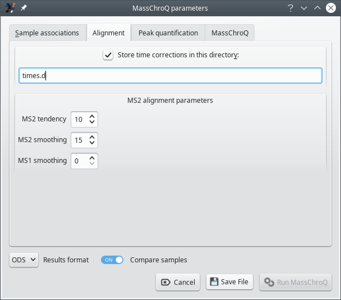
This tab configures the way i2MassChroQ performs the XIC chromatograms alignment between associated samples in the various groups. If the user is interested in the results of the alignment, the XIC retention time corrections can be stored in the directory specified at Store time corrections in this directory for later scrutiny.
Figure 7.7: The MassChroQ interface window (Alignment) #
The MS2 alignment parameters group box widget gathers parameters that are critical to the XIC chromatogram alignment algorithm for all the samples associated in a given group, as described below.
MS2 tendency: half size of the window used to apply a moving median on the MS/MS retention time deviation curve. Used to create the tendency deviation curve. Of course the appropriate value for this window depends on the number of identified peptides that the two runs (reference run and run being aligned) have in common. Usually a good value is 10. While aligning, MassChroQ outputs the number of peptides in common which can be used to readjust this parameter if necessary.
MS smoothing: half size of the window used to apply a moving average on the MS/MS retention time deviation curve. Smooths the deviation curve. Same as the above parameter, usually a good value is 10.
MS1 smoothing: half size of the window used to apply a moving median on the MS retention time corrections curve. This smoothing parameter is optional, and it is not necessary most of the time. It could be used in place of the MS2 smoothing parameter in cases of a small number of shared identified peptides (< 100), in which case a good value is 20.
7.1.2.3 The Peak quantification Tab #
This tab allows one to configure the way the peaks in the XIC chromatograms are evaluated from a quantification stand point. These parameters need some testing as they might depend on the instrument whence the data originated.
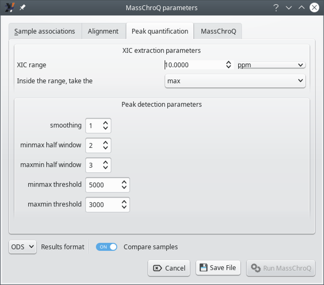
This tab configures the way i2MassChroQ performs the evaluation of the peaks in the XIC chromatograms from a quantification stand point. The settings in this dialog window might need some tweaking as they might depend on the instrument whence the data originated.
Figure 7.8: The MassChroQ interface window (peak quantification) #
XIC extraction parameters: these parameters govern the way the program searches for m/z values in the mass spectral data.
XIC range: the m/z width (mass tolerance) for searching m/z values in the mass data during the XIC extraction. Units can be part-per-million (ppm), resolution (res) or Dalton (dalton). The wider the window, the rougher the XIC extraction. This value typically depends on the resolving power of the instrument that acquired the data.
Inside the range, take the: once the m/z window has been located in the mass spectral data, it will contain a nubmer of points. This settings determines what kind of signal intensity to compute for the m/z window (that is, what to do with the m/z points contained in the m/z window). If maxis selected, only the max-intensity point in the m/z window is used as the signal intensity corresponding to the m/z window. If sum is selected, the sum of the intensities of all the m/z points in the window is used.
Peak detection parameters: these parameters govers the way the program detects peaks.
smoothing: number of points around the point being considered in the XIC chromatogram. If set to one, the rolling window will contain three points: one before the considered point, one after it and the considered point itself. This setting thus determines the width of the rolling window that is used to iterate in the XIC chromatogram in search for peaks. This window, whatever the setting, will shift by one point at each iteration in the XIC chromatogram.
minmax half window: the half window size used to apply the close (min/max) transform on the XIC intensities. This window determines the number of scan points over which two peaks will be considered separately, otherwise they would have been merged. A good half window value is usually 3 (which makes a window of 7).
maxmin half window: same as above but for the close (max/min) transform. This window determines the minimum peak width (in scan points number) below which the peak would not be detected. A good half window value is usually 2 (which makes a window of 5).
minmax threshold: threshold on the close signal: a minimum intensity value below which peaks are not detected on the closing signal. This threshold is usually two or three times the background noise intensity level, which depends on your mass spectrometer.
maxmin threshold: threshold on the open signal: a minimum intensity value below which peaks are not detected. It corresponds to the opening signal upper limit and it represents the background signal upper level. A good value would thus be slightly bigger than your background noise intensity level.
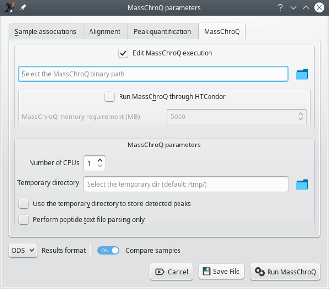
7.1.2.4 The MassChroQ Tab #
This tab allows one to configure the way MassChroQ actually performs the
quantification (if using the Run MassChroQ) or
the way i2MassChroQ writes the masschroqml file to be fed to the MassChroQ
program.
This tab configures the way either MassChroQ actually performs the
quantification or i2MassChroQ writes the masschroqml file that MassChroQ will be
fed with to perform the task.
Figure 7.9: The MassChroQ interface window (MassChroQ) #
Edit MassChroQ execution: activate the check button to use the directory icon to locate the MassChroQ program on disk. The full path to the program will be printed in the line edit widget next to the icon.
Run MassChroQ through HTCondor: activate the check button to set the memory requirements for HTCondor.
MassChroQ parameters: these settings govern the actual MassChroQ quantification process:
Number of CPUs: set the number of central processing units that MassChroQ is allowed to use (these are actually called “threads”).
Temporary directory: use the directory icon to select a specific temporary directory where MassChroQ will write processing-related data. By default the directory is
/tmp/. The temporary files are eliminated when no more used.Use the temporary directory to store detected peaks: if checked, the detected peaks might be stored in files in the temporary directory described above. This can be construed as a swap area where to store peaks data if the available memory is insufficient.
7.1.2.5 Saving the File and Optionally Running MassChroQ #
Once all the configuration has been done, the user can either only save
the masschroqml file by clicking
on the Save File button or immediately start
MassChroQ by clicking on the Run MassChroQ button.
Note
Even if the user decides to go down the direct Run
MassChroQ route, the program will ask to save the
masschroqml file. This is
because that file is read by MassChroQ when i2MassChroQ internally calls it to
run the quantification process.
The masschroqml file describes
the proteins and peptides that were retained during the protein
identification results analysis session. The contents of the file are
shown in Figure 7.10, “Contents of the masschroqml file”.
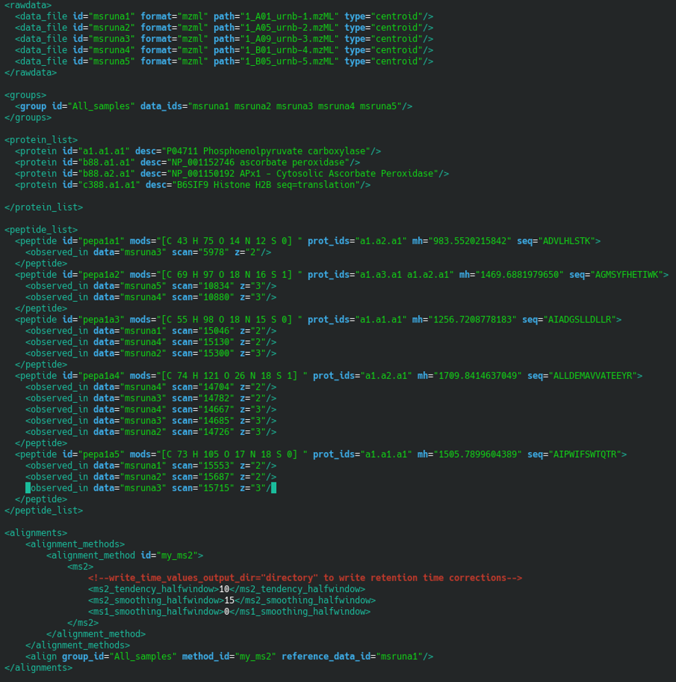
The masschroqml file
contains all the required data and configuration bits to perform
the XIC extractions for all the peptidic precursor ions that
allowed identifying proteins. This file is read by the MassChroQ
program. (In this screen dump, the file contents were obviously
redacted for brevity.)
Figure 7.10: Contents of the masschroqml file #
7.2 Interface to the MSstats Statistics Module #
The statistical analysis of the quantified peptide data by MassChroQ is assigned to the MSstats software authored by M. Choi and colleagues (2014) MSstats: An R package for statistical analysis of quantitative mass spectrometry-based proteomic experiments in Bioinformatics. As a prerequisite, peptide quantification must thus have been performed by MassChroQ as described in earlier sections.
This section describes in a step-by-step fashion the interface that i2MassChroQ provides to the MSstats software. To start the process, select the the menu item of the main menu, as shown in Figure 7.11, “MSstats menu item in the main i2MassChroQ menu”.
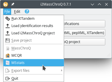
Menu that loads the interface to the MSstats statistics software that processes the MassChroQ-quantified peptide data to provide protein quantifications.
Figure 7.11: MSstats menu item in the main i2MassChroQ menu #
When the MSstats interface is loaded it looks like that shown in Figure 7.12, “Main MSstats interface window”. The actions to be carried over are shown on the left hand side region of the window in the form of a series of actions that are materialized by gradient-filled buttons. Each one of these actions are described in the following sections.
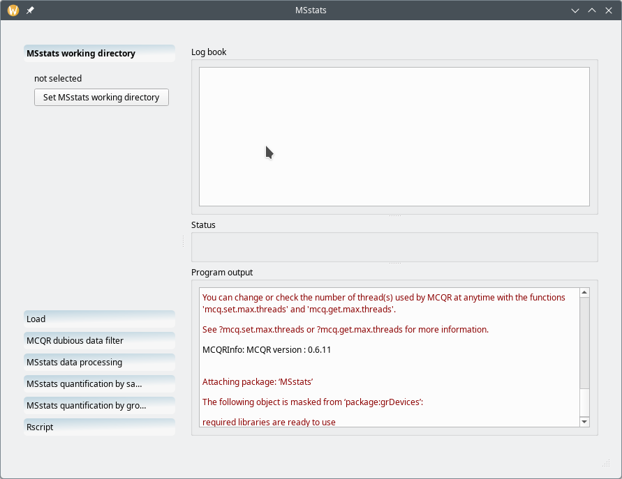
The main MSstats interface window has two main regions: the left hand side part of the window contains all the workflow steps that are to be carried out from the topmost item to the bottommost item; the right hand side part of the window contains three elements: the Log book view at the top, the Program output at the bottom, and the central Status widget.
Figure 7.12: Main MSstats interface window #
7.2.1 Setting the temporary MSstats working directory #
The first choice to be made by the user is to define where the MSstats package will write the data it needs to fulfill its statistical analysis tasks (Figure 7.13, “Setting the MSstats working directory”). The directory needs to be created if it does not exist already.
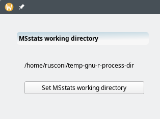
The directory is used by MSstats to store all the files and directories it creates during its fulfilling of its tasks. That directory can be located anywhere on the disk and needs to be created if it does not exist already.
Figure 7.13: Setting the MSstats working directory #
7.2.2 Loading the peptide quantification data file by MassChroQ #
The MassChroQ-based peptide quantification process must have been performed
already and must have produced an XML file with the masschroqml extension. That file can be
loaded by clicking the Select masschroqML file
button.
Upon completing the data file loading process, the right hand side pane of
the windows shows a summary of the data just loaded in the Log
book widget (Figure 7.14, “Loading MassChroQ-generated data file”).
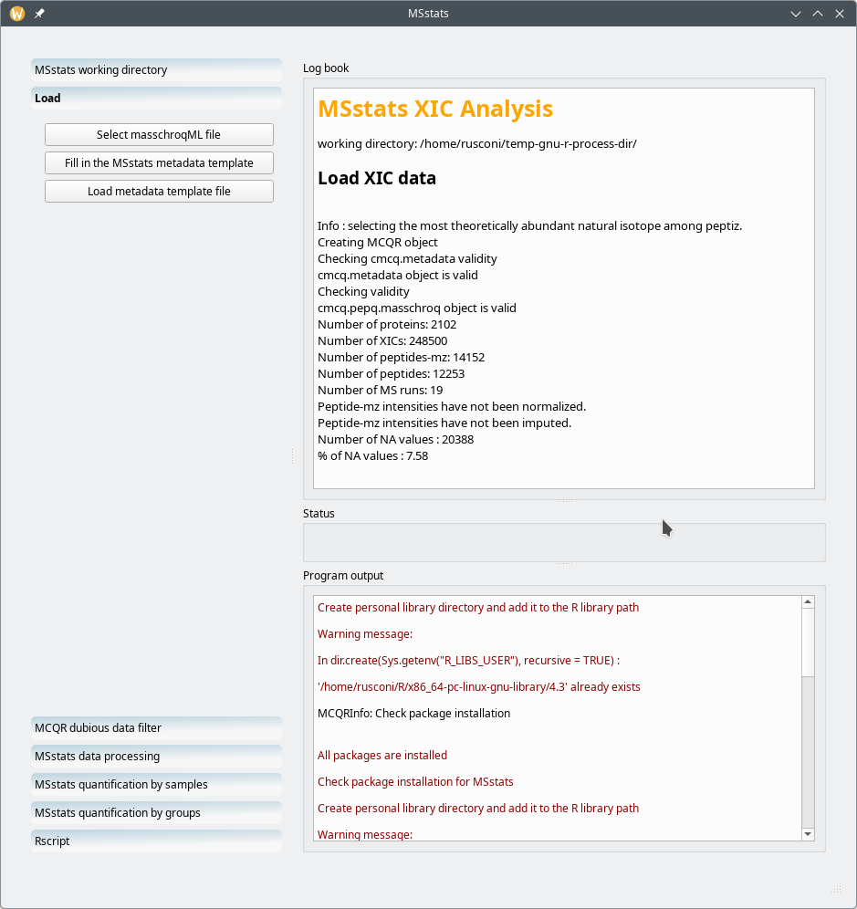
The peptide quantification process by MassChroQ produces a file that the user must load by clicking onto the Select masschroqML file button. As shown in the Log book pane on the right hand side of the window, the data have been loaded and a summary is provided.
Figure 7.14: Loading MassChroQ-generated data file #
Once the data have been loaded, i2MassChroQ crafts a brand new spreadsheet
data set in memory that needs to be stored on disk. For this, the user
clicks the Fill in the MSstats metadata template
button, which will permit saving the file to disk (with the OpenDocument
format, ods extension, typically in
the working directory created earlier). i2MassChroQ will try to automatically
open that file right after having written it to disk. If the file cannot
be opened, then user needs to open it manually and start filling in the
metadata for MSstats to performs its work as intended. A typical unmodified
metadata template file looks like shown in Figure 7.15, “Metadata template file for use by MSstats” where only the MS
run file names are listed.
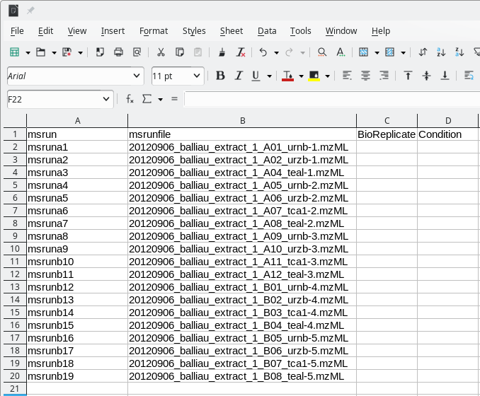
A typical MSstats metadata template file as created by i2MassChroQ. That file needs to be modified according the user requirements in terms of grouping the samples according to the experiment plan. When created, the file only contains the list of MS runs from which peptide quantifications were performed.
Figure 7.15: Metadata template file for use by MSstats #
Once modified by the user to annotate the MS run file names and to group the samples according to the experiment plant, the file looks like shown in Figure 7.16, “Annotated metadata for use by MSstats”.
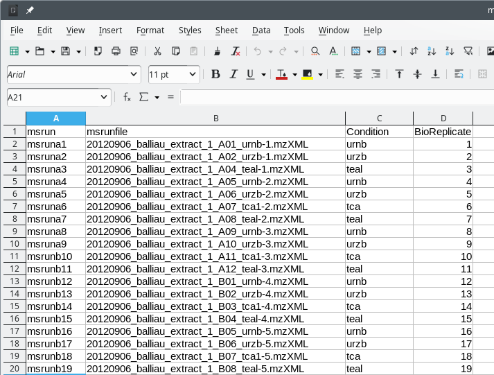
Once the template metadata have been completed to inform MSstats about the sample grouping and the analysis logic, it might look like shown in this figure.
Figure 7.16: Annotated metadata for use by MSstats #
The template file, as modified by the user should next be loaded by clicking on the Load metadata template file button. The Log book widget now shows informational data like shown in Figure 7.17, “Preliminary processing performed by MCQR upon loading of the metadata template file”. The output data are comprehensive and illustrated with graphs like the one described below.
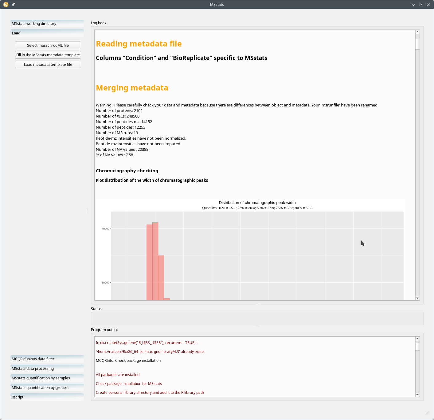
The template metadate file loading step triggers preliminary computing tasks by MCQR (a GNU R script developed in our facility) and the output is provided in the Log book widget.
Figure 7.17: Preliminary processing performed by MCQR upon loading of the metadata template file #
One particular informational bit that is of use in a later step of the processing workflow is the distribution of the chromatographic peak width over all the samples and over the whole retention time (Figure 7.18, “Chromatography data checks: the distribution of the chromatography widths”). Equally useful is the distribution of retention time variability for all the (m/z,z) pairs that were extracted from the whole set of MS run acquisitionsFigure 7.19, “Chromatography data checks: the distribution of retention time variations”.
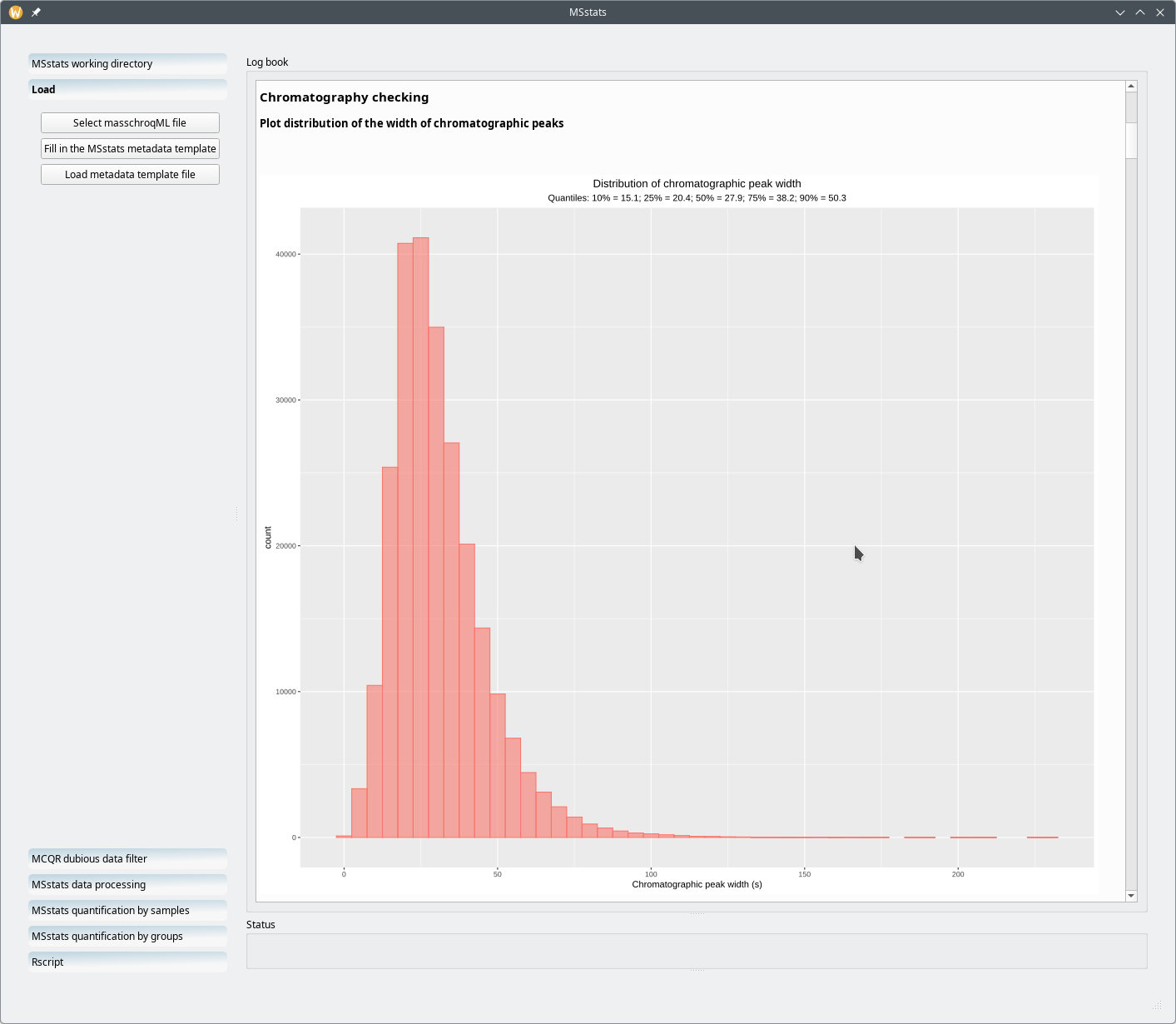
MSstats prints out data used by i2MassChroQ to plot a number of graphics like this histogram showing the distribution of the peak widths (in seconds). One can assume that a given ion might be reasonably contained in a retention time range (0—150) seconds.
Figure 7.18: Chromatography data checks: the distribution of the chromatography widths #
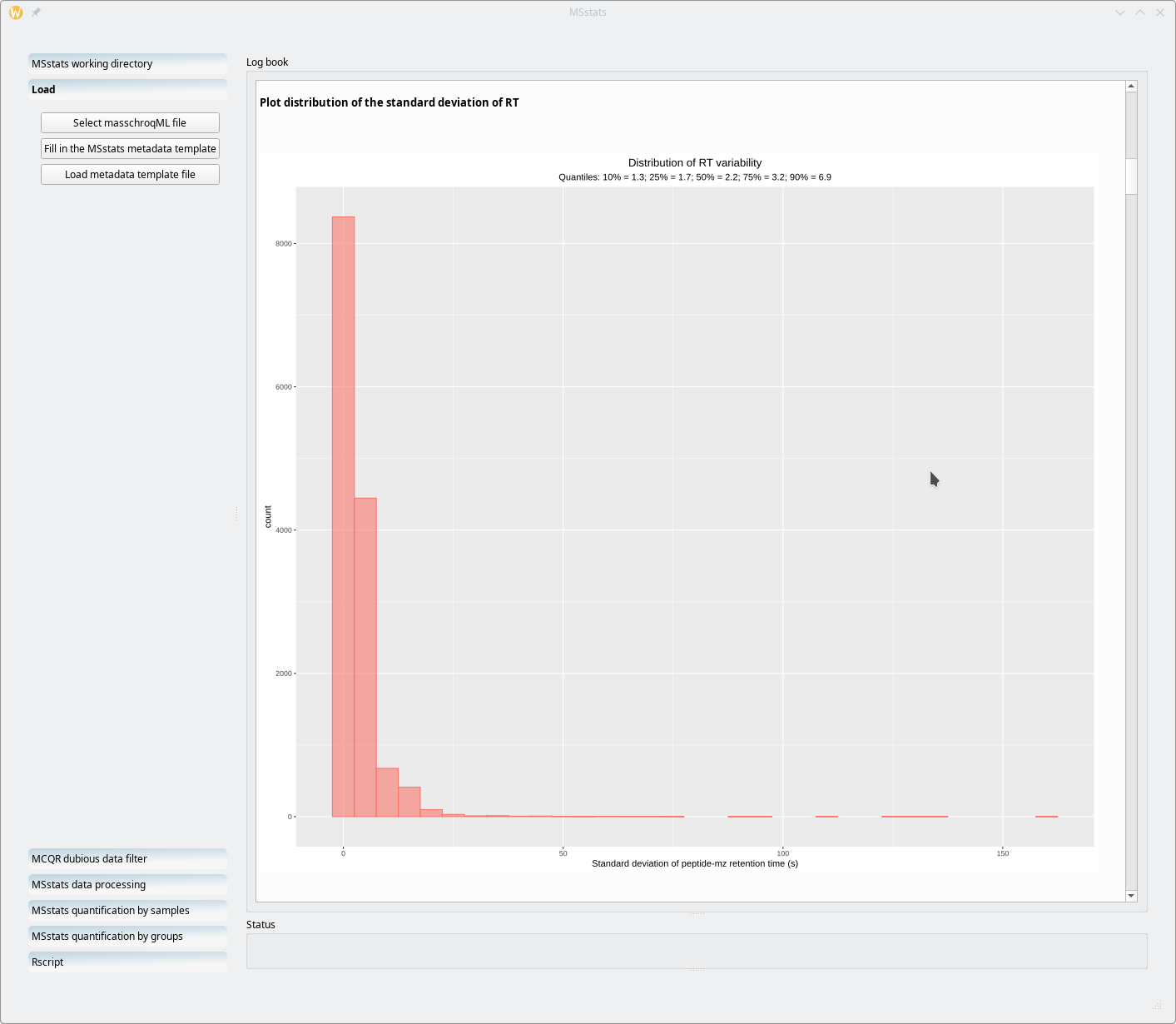
The histogram plot here shows the variability of the retention time values for all the (m/z,z) pairs extracted from the whole set of MS run acquisitions. One might consider that the maximum standard peak width variation acceptable is 30.
Figure 7.19: Chromatography data checks: the distribution of retention time variations #
The two information bits described in the two figures above are of use in the next step of the processing workflow, as described in the next section.
7.2.3 Filtering dubious data by running MCQR #
This step is optional. It is performed by MCQR. The idea is that the user should be able to scrap some dubious data from the data set if these data are outside of “reasonable ranges”. For example, one should be able to filter out (m/z,z) pairs if they match retention times of too large a range (that is, for example, an ion being detected in the MS run acquisition over too long a retention time range, which is suspect).
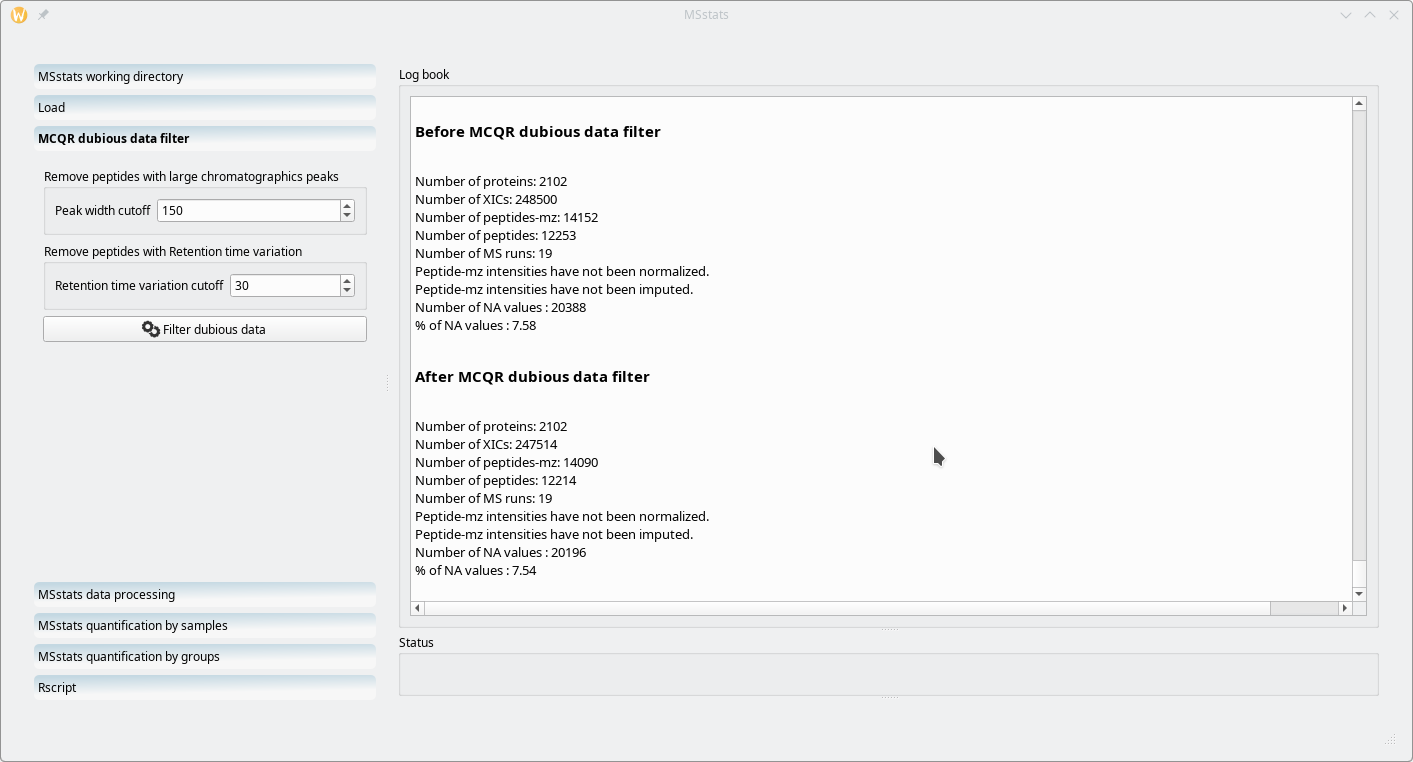
Dubious data might be filtered out on the basis of the two criteria shown. The numerical values set in this example are based on the output of MSstats as shown in the previous histograms.
Figure 7.20: Filtering dubious data using MCQR #
The dubious data filtering is performed on the basis of two criteria: the retention time peak width (Peak width cutoff) and the retention time variability (Retention time variation cutoff). i2MassChroQ documents the filtering step in the Log book widget as shown in Figure 7.20, “Filtering dubious data using MCQR”.
As visible in Figure 7.20, “Filtering dubious data using MCQR”, in the ouput printed in the Log book widget, the data set is pretty good, since applying the filters did only remove 39 peptides over more than twelve thousands and not a single protein.
7.2.4 Running MSstats on the configured data set #
The next step in the wokflow is to actually run MSstats. However, one last bit of configuration is required: the user is requested to select the log transformation (either log2 or log10) because that is a prerequisite for MSstats to run. Once that configuration bit has been set, the user might click on the Run MSstats button.
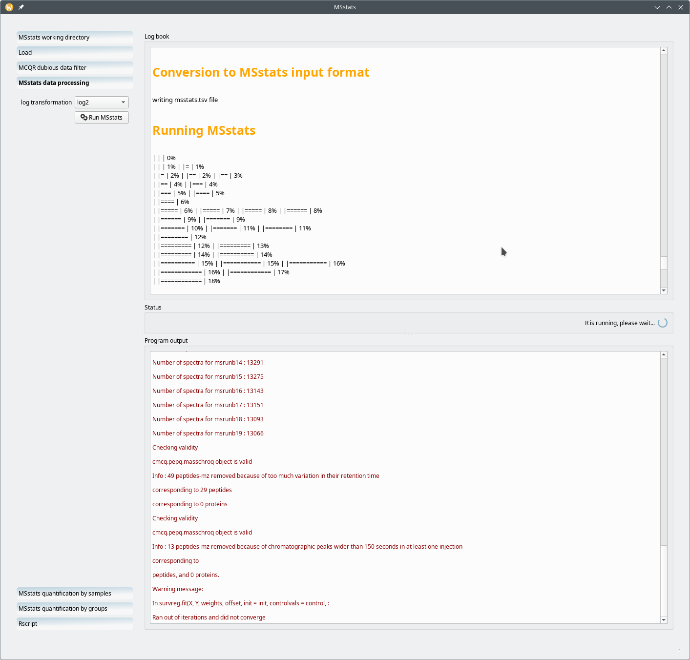
After having chosen the log tranformation (log2 or log10) that is required by MSstats, the user clicks on the Run MSstats button. The output shows the advancement of the computations.
Figure 7.21: Running MSstats on the configured data set #
At the end of the computation, as shown in Figure 7.21, “Running MSstats on the configured data set”, the starts the next workflow step.
7.2.5 Running the MSstats quantification by samples #
One of the manners in which the MSstats-based quantification process can be run is the “quantification by samples” mode. This is triggered by clicking on the MSstats quantification by samples workflow item, as shown in Figure 7.22, “MSstats quantification by samples mode”.
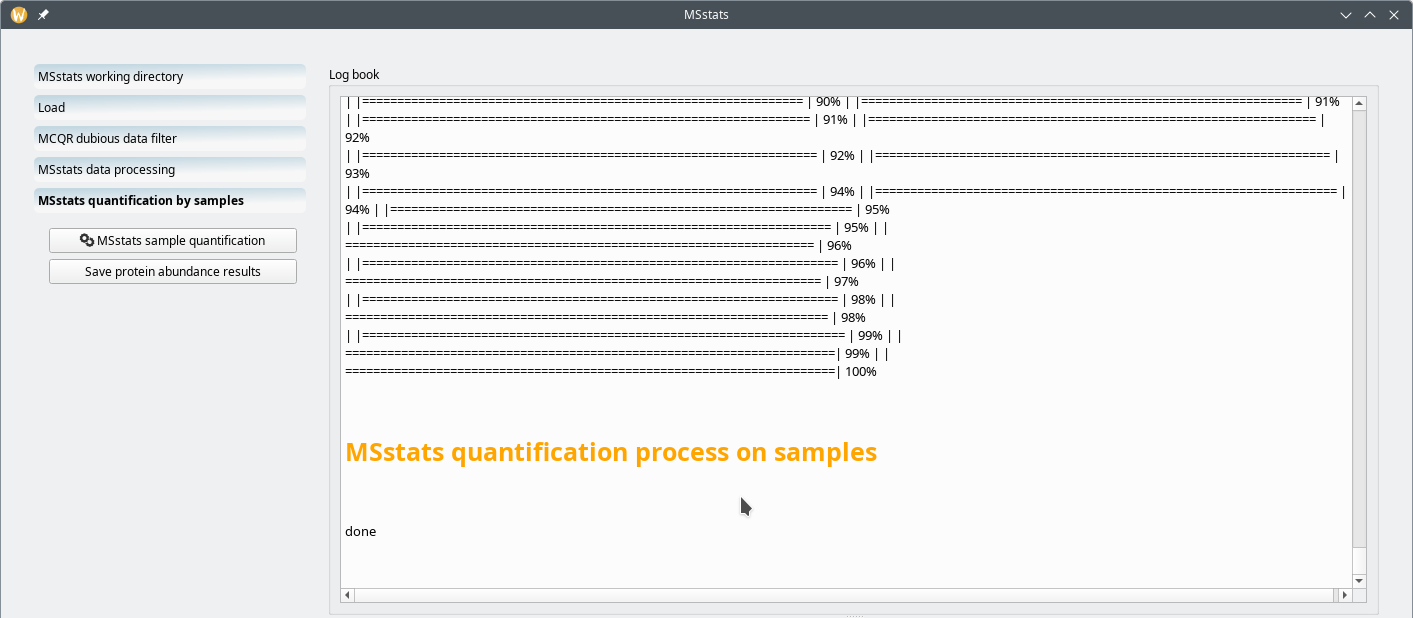
In the quantification by samples mode, the samples are taken as individual samples depending on their BioReplicate number in the metadata template file. See text for details.
Figure 7.22: MSstats quantification by samples mode #
The quantification process depicted in Figure 7.22, “MSstats quantification by samples mode” is very quick. The “processing by samples” mode will quantify protein on the basis of the “BioReplicate” variable in the metadata template file (Figure 7.16, “Annotated metadata for use by MSstats”). Because, in the example, each MS run acquisition (that is, each row of the spreadsheet page) is marked as a different BioReplicate, the quantification by samples mode will quantify proteins found in each individual sample separately.
The user will want to save the protein quantification results by saving them to a spreadsheet file. This step is achieved by clicking the Save protein abundance results button. The saved spreadsheet file is shown in Figure 7.23, “Spreadsheet view of the quantification by samples results”.
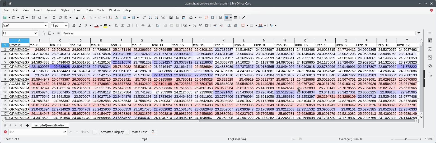
In the metadata template file, each MS run acquisition was listed as a different BioReplicate identity. This means that proteins were quantified independently in each MS run. The spreadsheet view in this figure shows quantification data for each protein (each row) found in each each sample (the columns).
Figure 7.23: Spreadsheet view of the quantification by samples results #
7.2.6 Running the MSstats quantification by groups #
The other manner in which the MSstats-based quantification process can be run is the “quantification by groups” mode. This is triggered by clicking on the MSstats quantification by groups workflow item, as shown in Figure 7.24, “MSstats quantification by groups mode”.
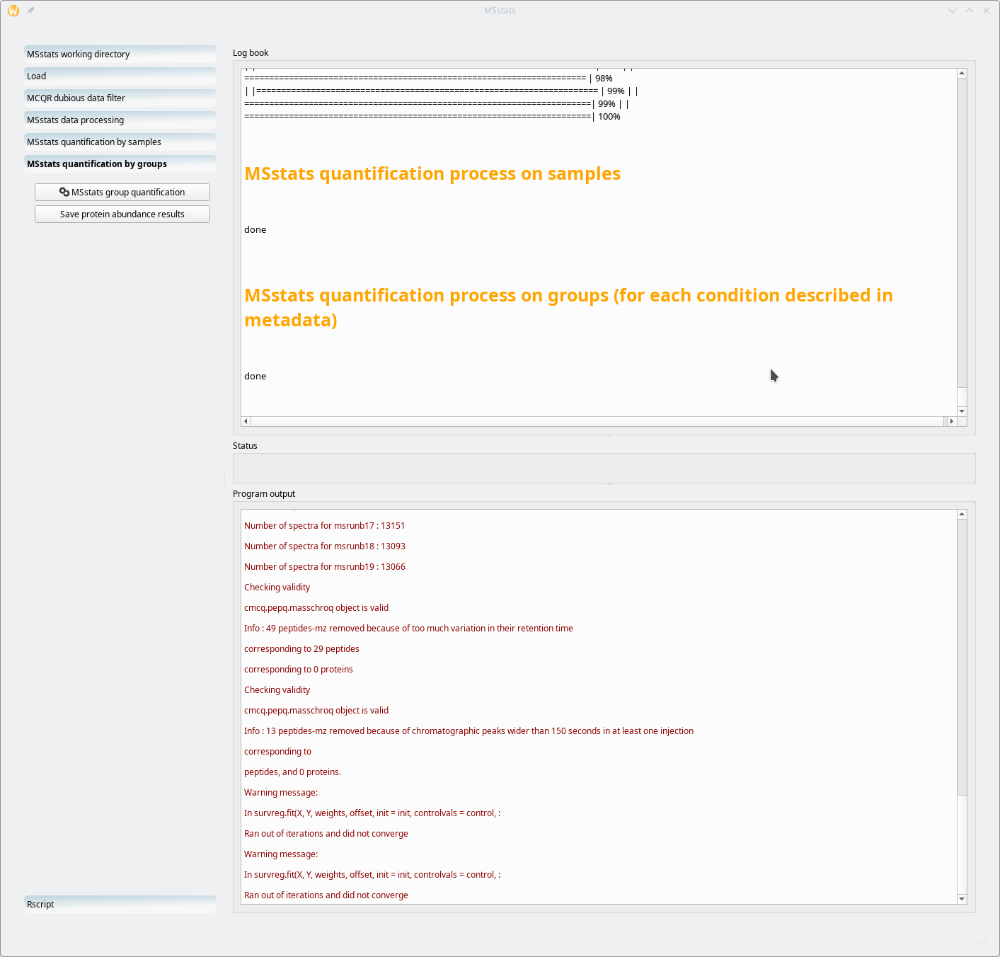
In the quantification by groups mode, the samples are first grouped into groups defined in the metadata template file. In that file, the column that specifies the required grouping has the Condition header. See text for details.
Figure 7.24: MSstats quantification by groups mode #
The quantification process depicted in Figure 7.24, “MSstats quantification by groups mode” is very quick. The “processing by groups” mode will quantify proteins on the basis of the “Condition” variable in the metadata template file (Figure 7.16, “Annotated metadata for use by MSstats”). Because, in the example, there are four different Condition values, there will be four groups of proteins (different protein solubilization methods).
The user will want to save the protein quantification results by saving them to a spreadsheet file. This step is achieved by clicking the Save protein abundance results button. The saved spreadsheet file is shown in Figure 7.25, “Spreadsheet view of the quantification by groups results”.
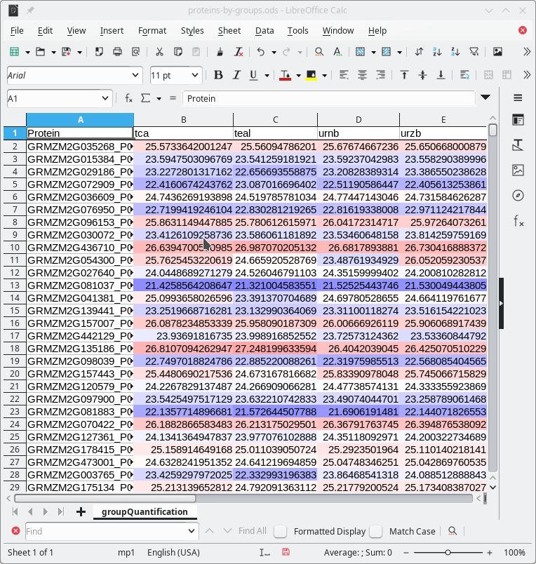
In the metadata template file, MS run acquisitions were grouped using the value of the Condition variable. The grouping of the MS runs involve thus four groups (different protein solubilization methods). This means that the proteins will be quantified in each group of MS run acquisitions.
Figure 7.25: Spreadsheet view of the quantification by groups results #
7.2.7 Running the MSstats GNU R and RMarkdown scripts #
The workflow as has developed since the beginning to this MSstats work session has been recorded both in the form of a pure GNU R script and as a RMarkdown script. By clicking onto the Rscript workflow item (Figure 7.26, “Load the GNU R and RMarkdown scripts”), the user is presented with two options: load the GNU R script and/or the RMarkdown script. The RMarkdown script might be run in the RStudio (RStudio has changed its name to become Posit) environment.
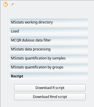
Use the button of interest to download the GNU R or the RMarkdown script corresponding to all the workflow steps that were run up to this one.
Figure 7.26: Load the GNU R and RMarkdown scripts #
Upon saving the RMarkdown version of the script, if available on the system, i2MassChroQ will try to load it automatically in RStudio.