mineXpert2 User Manual
2 The program's graphical user interface
Data exploration, in mass spectrometry, entails, for a large part, the relentless scrutiny of the mass spectra by an expert eye. Without a powerful mass spectrum viewer, capable of numerous data display modes, the expert eye remains powerless. In this chapter, the graphical user interface is described in detail, starting from the opening of a mass spectrometry data file, to the navigation through all the data depth within a large set of graphical representations of the data.
2.1 Opening Mass Spectrometry Data Files #
To start a session, open one or more mass spectra using the menu
→
menu. mineXpert2 understands the mzML, mzXML and MGF formats. The file
loading procedures, for these formats, are delegated to the excellent
libpwiz library from the
ProteoWizard project.[7]
Simple txt, asc data where m/z and intensity values are separated
by any character that is neither a newline nor a dot nor a digit
(loading is handled by a private parser) can be loaded either from file
or directly from the clipboard.
There are two variants of the mass spectrometry file opening menu, one for which the mass data are read from file and stored totally in memory and one for which the mass data are read from file in streamed mode, used to compute the TIC chromatogram and discarded. The latter mode is useful when the mass data are so large that they cannot fit in memory. Optionally, a table view can be displayed with all the data in the MS run data set that was loaded from disk. The TIC chromatogram or the table view can then be used to access the mass data in the file according to criteria set by the user (retention time range, for example).
2.2 The Window Layout #
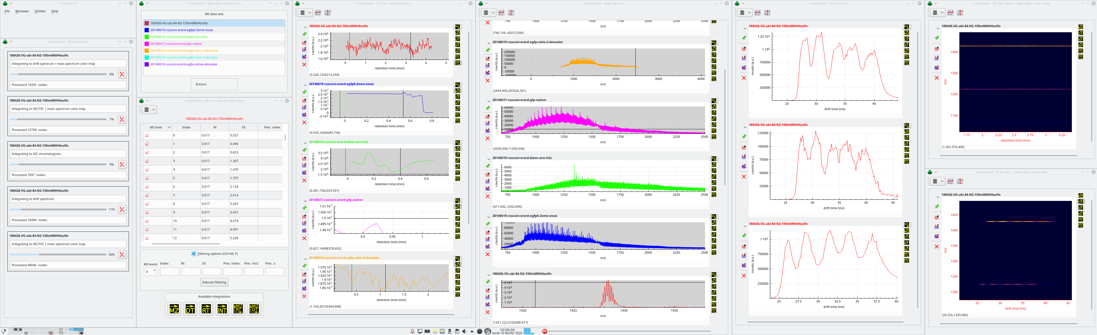
The graphical interface of comprises a number of windows where data and informations are displayed. When first started, the program shows the main program window. Upon loading of a MS run data set from file, new windows do show up as described below (see Figure 2.1, “General View of the Graphical User Interface”):
mineXpert2 main program window: this is an unintrusive window sporting the main menu;
The Task monitors window, that displays all the ongoing tasks, always providing the user the ability to cancel an ongoing task;
The Open MS run data sets window, that lists all the mass spectrometry data sets that have been loaded from file;
The TIC/XIC chromatograms window[8] where the various TIC/XIC chromatograms are displayed for the various mass spectrometry data files that have been loaded. There is, by definition, a single TIC chromatogram for each MS run data set currently loaded in the program. However, this window will also display ion current chromatograms that are computed as a result of an integration step from the other windows, like from the Mass spectra window or from the Drift spectra window. In this case, the chromatogram is an extracted ion current chromatogram (XIC chromatogram);
The Mass spectra window, where the various mass spectra are displayed. A given mass spectrum may originate from a TIC chromatogram, from the MS run data set tableview window, from a drift spectrum, or even from a color map;
The Drift spectra window, where the various drift spectra are displayed. Like stated before, drift spectra can originate from a variety of places;
The TIC/XIC chrom. /Mass spec. color maps window, that contains int = f(rt, m/z) color maps, two-dimensional representations of the relation between the retention time and the mass spectral data. The intensities are represented as colors in a gradient map;
The Drift spec. /Mass spec. color maps window, that contains int = f(dt, m/z) color maps, two-dimensional representations of the relation between the drift time and the mass spectral data (in ion mobility mass spectrometry experiments only). The intensities are represented as colors in a gradient map;
The Console window, where the various messages or analysis data elements are displayed for the user to select, copy and paste in an electronic lab-book;
The position and size of all the windows can be stored for a later session
Figure 2.1: General View of the Graphical User Interface #
2.3 The Main Program Window Menu #
The menu bar in the main program window displays a number of menu items, reviewed below:
→ : Select the mass spectrum file(s) to load. The mass spectral data read from disk are stored in memory. This means that if the file is greater than the available system memory (RAM), the user is urged to select the next menu;
→ : Select the mass spectrum file(s) to load. The mass spectral data are read from disk, the TIC chromatogram and the MS run data set statistics are computed and then the data are freed. This file opening mode is compulsory when the mass data file is larger than the available system memory (RAM);
→ : Create a mass spectrum from a textual representation of (m/z,i) pairs in the same format as described above for the txt,asc file format;
→ : Set the preferences for the exploration results storage;
The menus are self-explanatory, as they explicitely explain which window is to be shown. The menu records on disk the position and size of all the windows, so that upon reopening the program, the windows all position themselves at the recorded position and size;
→ : Open a dialog window to set up XIC extractions for any one of the currently loaded mass spectral data set;
→ : Open the window in which the isotopic cluster calculations are configured and run;
→ : Open the window in which the mass peak shape calculations can be configured and run.
→ : Set the maximum number of execution threads that mass spectral integrations can use. Note that the program starts to be really efficient with a number of threads at least equal to 4 (see Section 1.5.3, “Using multiple threads during mass data integrations”).

Tip
Do not mistake “thread” for “core” or “processor”. When processors are described, the description usually says “x core”. That means that there are x “processors” in the whole central processing unit attached to the motherboard. Each processor most often can branch two different threads. So a computer that sports 2 cores, will most often in fact make 4 threads available for the computations.

Warning
It is of utmost importance to make sure that guest virtualized environments do share at least 2 (better 4) threads with the host system. In VirtualBox, for example, it is possible to allocated a defined number of threads to the guest operating system. Ensure that the number of threads made available to the guest operating system is at least , with 4 being a right low level value.
This menu's items show help about the program itself and also about the Qt libraries that were used to build it. These informations are essential in case the user wants to make a bug report.
2.4 The Loaded MS Run Data Sets #
Each time a new MS run data set is loaded from disk or from clipboard, a corresponding MS run data set item is added to the Open MS run data sets dialog window (see Figure 2.2, “The open MS run data sets”).
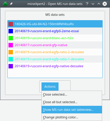
Each time a new MS run data set is loaded, a corresponding item is added to the list widget. The drop-down menu lists a number of actions that can be performed with these items.
Figure 2.2: The open MS run data sets #
One of the most useful menu items available from the drop-down menu of Figure 2.2, “The open MS run data sets” is the item. That menu item triggers the display of a window containing a table view, like in a spreadsheet, that shows the data of each scan contained in the MS run data set loaded from file. This window is described in the following section (see Figure 2.3, “The table view-based scrutiny of one MS run data set”).
2.5 Mass Spectral Data Listing in a Table View #
From the Open MS run data sets dialog window, it is possible to select one list widget item corresponding to the data set of interest and select the menu item that opens the MS run data set table view window shown in Figure 2.3, “The table view-based scrutiny of one MS run data set”.
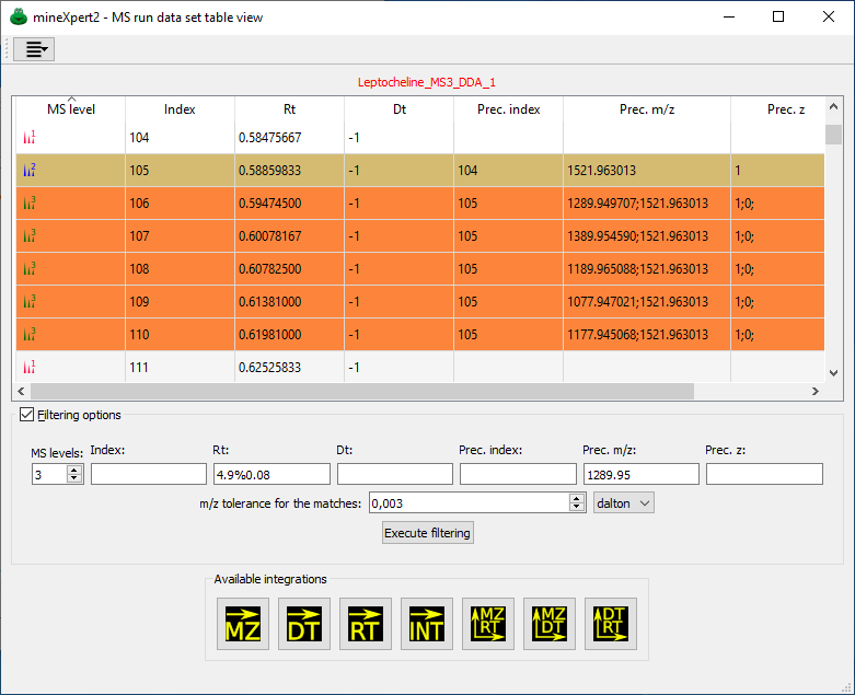
Each MS run data set might be scrutinized through the use of this table view. Each filtering criterion has a number of data insertion modalities, described in the text. In this example, the user has set a number of values in the Filtering options group box but has not yet executed the filtering, so the full mass spectral data set is listed in the table view.
Figure 2.3: The table view-based scrutiny of one MS run data set #
The data that belong to each spectrum in the acquired mass spectral data set are shown as values in dedicated columns. Each row represents a mass spectrum of the data set. There might be tens of thousands spectra in an acquisition. Note that two columns may contain ;-separated values. These columns are Prec. m/z and Prec.z, respectively precursor ion m/z and precursor ion charge. Ions of differing m/z values and of differing charge values might be accumulated in a trap and then fragmented in a single fragmentation step. The mass data file thus contains spectra with a list of selected precursor ions.
Note
When multiple values are listed in precursor m/z and charge cells, these value behave as if they were alone in the cell. When performing filtering of the data (see below), then the program treats each value of the list as if it were alone in the cell. For example, in Figure 2.4, “Mass spectral data set filtering using combined criteria” the user filtered the MS data on the basis of a Prec. m/z value of 1289.95. That filter selected the row that lists, as Prec. m/z, the value 1289.952393;1521.973633.
In the MS run data set table view window, the checkable group box labelled Filtering options allows one to open a series of widgets in which to set the values for various filtering criteria.
MS levels: Set 0 to retain all the mass spectra, irrespective of their MS level. Enter value 1 to filter out any MS level that is not 1. This fields has no practical limit, allowing one to perform MSn data exploration.
Index: Filter by the index number of the mass spectra. This may be of interest when the indices are somehow known in advance.
Rt: Filter by retention time, that is, the time at which the mass spectrum was acquired, relative to the start of the mass data acquisition.
Dt: Filter by drift time (ion mobility mass spectrometry generates this kind of data).
Prec. index: Precursor index.
Prec. m/z: Precursor charge.
The general syntax used to fill-in the filtering options is according to the following scheme:
simple value, like 1 for MS levels.
<value: keep rows where values are less than the entered value.
>value: keep rows where values are greater than the entered value.
>start <end: keep rows where values are in between startand end. The match is not inclusive.
start--end: like before, but the match is inclusive. Mind the double-dash that delimits the values of the range.
value%tolerance: equivalent to the preceding item, unless start is (value- tolerance) and end is (value + tolerance).
Warning: The specific case of precursor m/z values
When inserting a m/z value, there is a specific tolerance widget m/z tolerance for the matches that allows one to define the tolerance with which the matches for the precursor m/z values are performed. That mechanism does not override the value%tolerance value definition modality described above; instead, it will add another tolerance to the range values.
Once the filtering values have been entered and validated by clicking or by keying-in Ctrl–ENTER, the items (that is, the table rows) that verified the filter, still present in the table view, might be selected (all of them or only some of them) for their integration to a variety of destinations. The destination of each integration is selected by clicking the proper icon push button from the button row below. The meaning of these push buttons will be described later (see Section 2.7.2, “The Right Column of Buttons Configures the New Integration to Run”).
Tip
Make sure to set the m/z integration parameters before performing an integration to a mass spectrum. The setting dialog window opens up using the menu item from the window's main menu, at the top left corner of the window. If the bin size value is too small, the integration might last very much longer than for a “reasonable” size.
The user might enter as many filtering criteria as necessary to pin point the most elusive feature in the mass spectral data set. In Figure 2.4, “Mass spectral data set filtering using combined criteria”, the user has filtered the data to retain MS3 mass spectra obtained by fragmenting ions of a given m/z value using a specified tolerance for the m/z match in Dalton units.
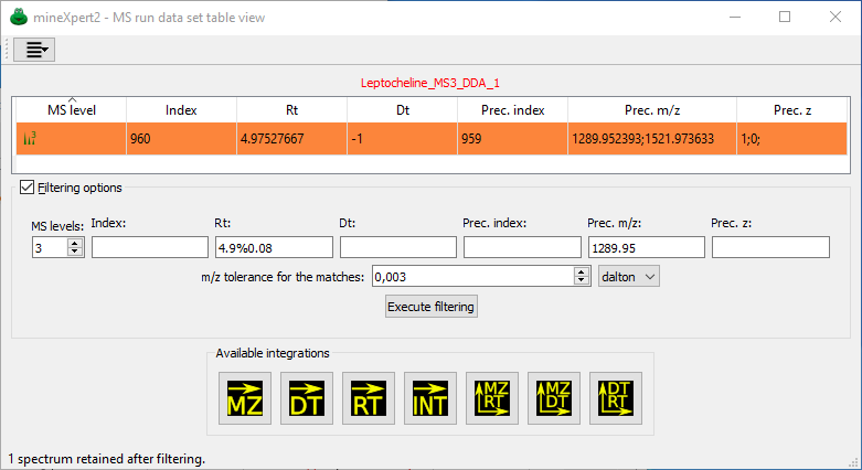
The use of combined filtering criteria allows one to pin point elusive mass spectral features.
Figure 2.4: Mass spectral data set filtering using combined criteria #
2.6 The Main Data-Plotting Windows #
This section will succinctly describe the main data windows of mineXpert2. Each window will be described in greater detail when the features of the program will be described.
Tip
Although not visible, the various plot widgets in the various plot windows are glued together with splitters that allow their resizing if the window becomes too crowded, as shown in Figure 2.5, “Resizing the plot widgets with the splitter”.
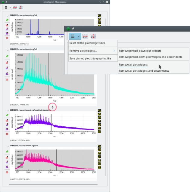
When positioning the mouse cursor between two plot widgets, the cursor switches to the splitter cursor shape (circled in red). Dragging that cursor will widen/shrink the plot widgets. To reset the plot widgets as they were initially created, use the from the main window menu shown on the right.
Figure 2.5: Resizing the plot widgets with the splitter #
As visible in all the figures of the plot widget-containing windows described in the next sections, the general structure of these windows is to have a menu in the toolbar, icon buttons in that same toolbar and then plot widgets stacked below in the order in which they have been created.
Note: The multi-graph plot widget has gone
In the first version of mineXpert the plot window was divided in two parts; the upper part had a plot widget in which all the plots were overlaid, the lower part had as many plot widgets as there had been integrations because each plot widget could only have one plot in it.
This is no more true now, because, as will be described later, it is now extremely easy to duplicate any plot into any plot widget so as to overlay any number of plots into any number of plot widgets.
2.6.1 The TIC Chromatogram Window #
Each time a new mass spectrum file is loaded, its corresponding TIC chromatogram is computed and then displayed in a new plot widget in the TIC/XIC chromatogram window (Figure 2.6, “The total ion current (TIC) chromatogram window”). That window is indeed specialized in the plotting of TIC or XIC chromatograms. Each new TIC chromatogram plot that is generated as a result of the loading of a mass spectrometry data file is plotted using a new color. That color encodes the filiation of the whole set of plots that are generated while performing various integrations starting from that initial TIC chromatogram plot. For example, a red TIC chromatogram plot that serves as the starting point for a mass spectrum integration triggers the creation of a new mass spectrum trace plot that is plotted in red color. For color map windows, where there is not trace plot, the axis and tick labels of the plot are of the same color as that of the initial TIC chromatogram plot.
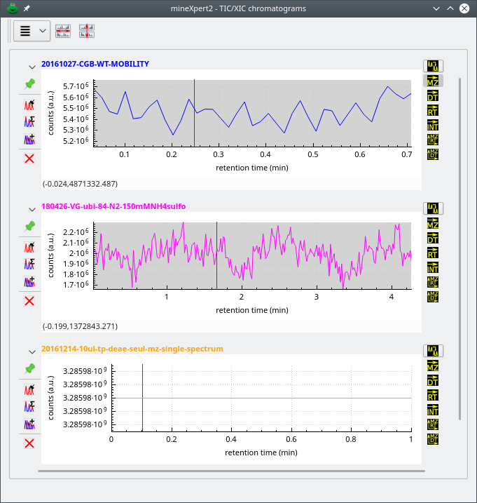
As many traces as necessary can be shown in the window. Each plot has its own set of crosshair markers.
Figure 2.6: The total ion current (TIC) chromatogram window #
Warning: Unconventional situations while loading mass spectrometry data files
When the user loads mass spectrometric data from a non-profile acquisition data file or from clipboard data, like when a mass spectrum is opened from a txt,asc,xy text-based format file where the data correspond to a single spectrum, not a sequence of spectra, the TIC chromatogram really has a single (rt,i) pair denoting the TIC intensity at the single retention time of that very unique spectrum. The TIC chromatogram window thus artificially creates and displays a TIC chromatogram that is a simple line, like shown in the bottom TIC chromatogram plot of Figure 2.6, “The total ion current (TIC) chromatogram window”. From there, integration happens like in conventional situations. Make sure that the mouse drag movement encompasses the whole TIC region by first unzooming a bit the trace.
When loading data files that only contain MSn data (n > 1), like the proteomics-oriented Mascot generic files (MGF), mineXpert2 cannot compute a TIC chromatogram. Indeed, a TIC chromatogram can only be computed for MS data, not MSn data. In this case, the TIC chromatogram plot that is created does not contain any plot. The only way the user can start exploring such kind of MSn (n > 1) data is by using the MS run data set table view window (Section 2.5, “Mass Spectral Data Listing in a Table View”).
2.6.2 The Mass Spectrum Window #
The mass spectrum window is specialized with the plotting of mass spectra. It thus contains all the plot widgets that display all the mass spectra that were created as a result of mass spectral data integrations. These integration might have originated in any plot widget of any kind (mass spectrum, drift spectrum, color map, for example). For example, the user might select a region in a TIC chromatogram and then ask that a mass spectrum integration be computed. In this case, the resulting mass spectrum is displayed in a new plot widget that is located in the mass spectrum window (Figure 2.7, “The mass spectrum window”).
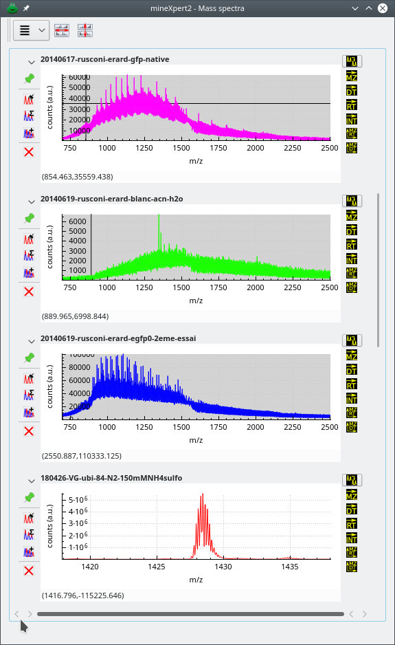
This mass spectrum window shows multiple mass spectra.
Figure 2.7: The mass spectrum window #
2.6.3 The Drift Spectrum Window #
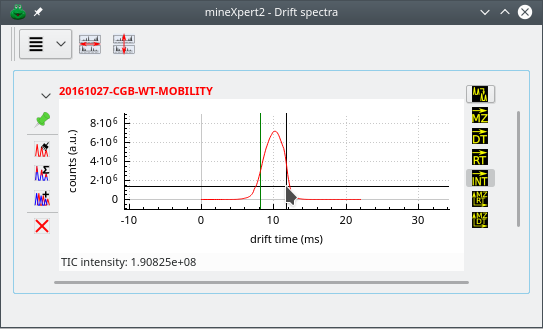
As described for the mass spectrum window, the drift spectrum window contains all the plot widgets that display drift spectra (Figure 2.8, “The drift spectrum window”).
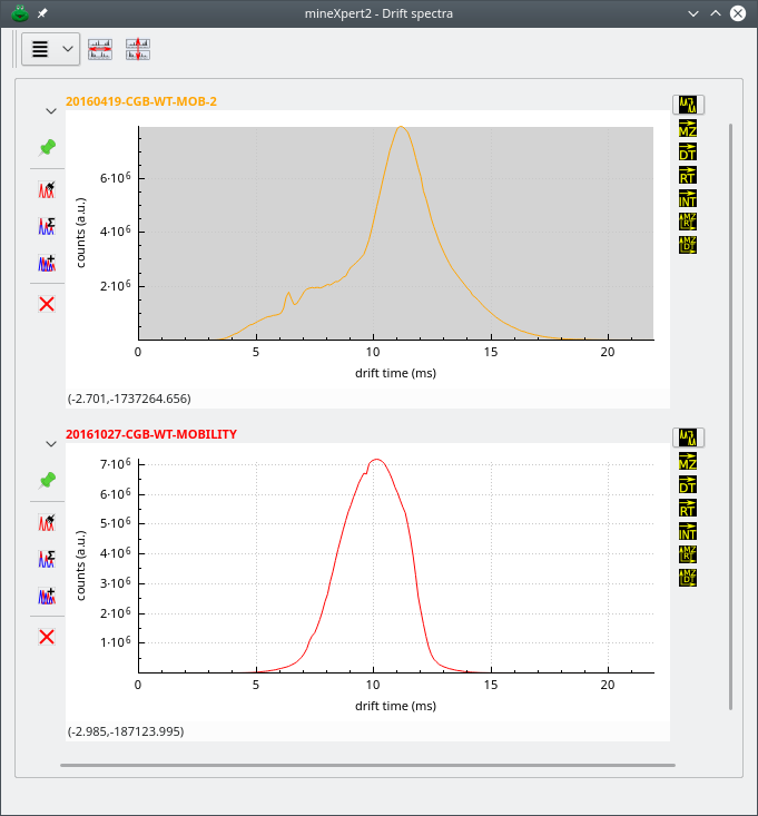
This drift spectrum window shows multiple drift spectra.
Figure 2.8: The drift spectrum window #
2.6.4 The Retention Time vs Mass Spectrum Color Map Window #
The int = f(rt, m/z) color map window displays a heat map relating all the retention time values with the corresponding mass spectra (see Figure 2.9, “The int = f(rt, m/z) color map window”). The window main menu offers menus that are all self-explanatory. The tool bar sports three buttons that:
Lock the x-axis of all the plot widgets in the window (first button).
Lock the y-axis of all the plot widgets in the window (first button).
Transpose the axes of the all the plot widgets that are pinned-down (see Note: The expression “pinned-down widget”).
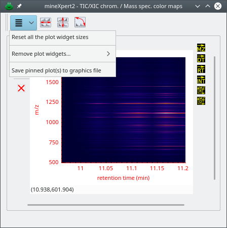
The mass spectrum vs retention time color map window relates mass spectra (y-axis) to retention times (x-axis).
Figure 2.9: The int = f(rt, m/z) color map window #
2.6.5 The Drift Time vs Mass Spectrum Color Map Window #
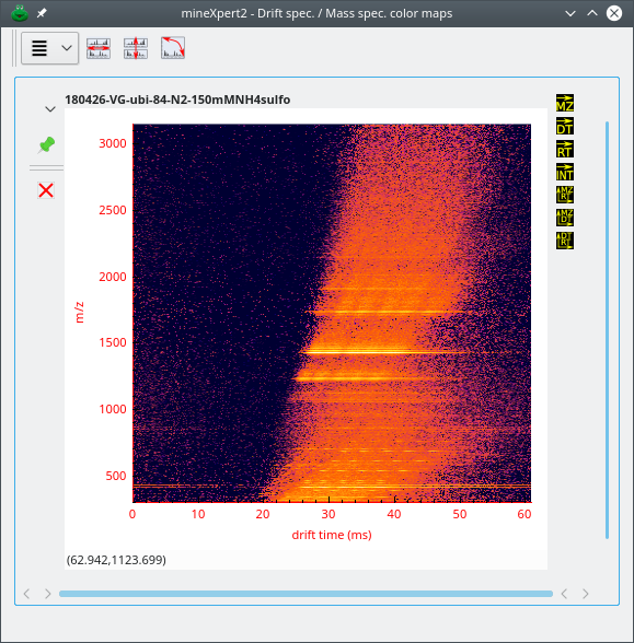
The int = f(dt, m/z) color map window displays a heat map relating all the drift time values with the corresponding mass spectra (see Figure 2.10, “The int = f(dt, m/z) color map window”).
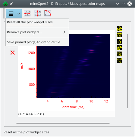
The mass spectrum vs drift time color map window relates mass spectra (y-axis) to drift times (x-axis).
Figure 2.10: The int = f(dt, m/z) color map window #
2.6.6 The Drift Time vs Retention Time Color Map Window #
The int = f(rt, dt;) color map window displays a heat map relating all the drift time values with the corresponding retention time values (see Figure 2.11, “The int = f(rt, dt) color map window”).
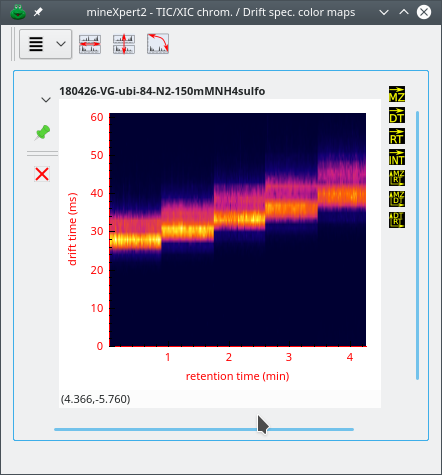
The drift spectrum vs TIC chromatogram color map window relates retention times (y-axis) to drift times (x-axis).
Figure 2.11: The int = f(rt, dt) color map window #
2.7 General Structure of the Plot Widgets #
The TIC/XIC chromatograms, mass spectra, drift spectra, retention time vs mass spectrum and drift time vs mass spectrum color map windows (collectively called plot widget windows) are all structured in a similar way as described below.
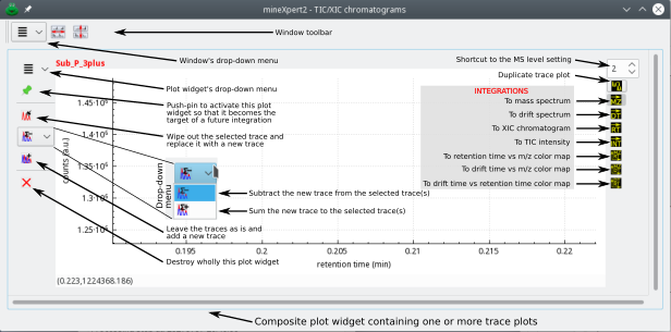
A composite plot widget is a widget that contains a number of other widgets. These sub-widgets are described.
Figure 2.12: Description of the various widgets that make a composite plot widget #
The window in Figure 2.12, “Description of the various widgets that make a composite plot widget” contains a single composite plot widget. Each composite plot widget's plotting area is sided by two columns of icons, which really are, for most of them, check buttons. The buttons in the left column configure if and how this plot widget is going to be the receiving container of a new integration result (result that takes the form of a trace plot). The buttons in the right column configure what kind of integration is to be performed using, as a starting point, one of the plots of this plot widget. Indeed, as already mentioned above, integrations in any plot widget might be configured to generate any kind of data: a XIC chromatogram, a mass or drift spectrum… If the data generated by a given integration constitute a XIC chromatogram, that chromatogram will be plotted in the TIC/XIC chromatograms window. Both columns of buttons (left and right) are detailed in the next section because these constitute the basis of the operation of mineXpert2.
2.7.1 The Left Column of Buttons Configures the Reception of a New Plot #
For this description, we will assume that the user is working in the TIX/XIC chromatograms window and is performing a new integration to a mass spectrum. The result of that new integration is thus a plot that needs to be installed in the Mass spectra window, as depicted in Figure 2.12, “Description of the various widgets that make a composite plot widget”. Such a window, however, might already contain a number of plot widgets; it is thus necessary to establish where the new plot is going to be created and how it will be created. These two questions are answered in detail below by describing the widgets in the left column of widgets in a composite plot widget.
The plot widget's drop down menu (downward arrow) will be described in detail later. The menu options are actions that apply to the plot widget that owns the menu;
 The push-pin button, if it is pushed
(therefore colored in red
The push-pin button, if it is pushed
(therefore colored in red  ), indicates
that the plot widget “claims” to be the receiving
container for any new integration destined to the window containing
it.
), indicates
that the plot widget “claims” to be the receiving
container for any new integration destined to the window containing
it.

Note: The expression “pinned-down widget”
A plot widget having its push-pin pushed down is said to be pinned-down. This is a terminology that will be used extensively in the rest of this manual.
If the window contains more than one plot widget and if more than one plot widget are pinned-down (
),
then all these plot widgets claim to be the receiving container of any new
plot to be installed in the window. If no plot widget in a window is
pinned-down, any new plot will be created in its own composite plot widget
that will appear at the bottom of the plot widget window.
In the list items below, we assume that the plot widget containing the various check buttons is pinned-down and belongs to a non-color map plot window.[9]
Checking the
 check button
indicates that the new plot will replace any selected
plot in the plot widget.
check button
indicates that the new plot will replace any selected
plot in the plot widget.
Checking the
 or the
 check button
indicates that the new plot will be subtract-combined
or add-combined from or into any selected plot in the
plot widget. This feature is particularly useful when trying a step-wise
estimation of the mass spectral data out of discrete discontinuous features
like TIC chromatogram peaks or drift spectrum peaks. Likewise and
reciprocically, it might be useful to extract, from different mass spectral
features in a given mass spectrum, the combined TIC chromatogram for them.
Typically, when an analyte appears in a mass spectrum under different charge
states that are separated by non-baseline regions, being able to assess the
XIC chromatogram for them in a series of combined integrations is extremely
useful. The subtract-combination is typically used for removing background
from a given trace using other blank trace as the background level.
check button
indicates that the new plot will be subtract-combined
or add-combined from or into any selected plot in the
plot widget. This feature is particularly useful when trying a step-wise
estimation of the mass spectral data out of discrete discontinuous features
like TIC chromatogram peaks or drift spectrum peaks. Likewise and
reciprocically, it might be useful to extract, from different mass spectral
features in a given mass spectrum, the combined TIC chromatogram for them.
Typically, when an analyte appears in a mass spectrum under different charge
states that are separated by non-baseline regions, being able to assess the
XIC chromatogram for them in a series of combined integrations is extremely
useful. The subtract-combination is typically used for removing background
from a given trace using other blank trace as the background level.
Checking the
 check button
indicates that the new plot will be added to the plot widget, that is, it
will be overlaid on top of any other plot in the plot widget.
check button
indicates that the new plot will be added to the plot widget, that is, it
will be overlaid on top of any other plot in the plot widget.
2.7.2 The Right Column of Buttons Configures the New Integration to Run #
Each plot widget may contain zero or more plots (also called graphs or traces). As mentioned earlier, any plot can serve as the starting point for a new integration to the same or another kind of data. For example, from a plot in the TIC/XIC chromatograms window, one might want to integrate a given retention time range to a mass spectrum or to a drift spectrum. How are those destinations determined ? The destination of an integration is selected by pressing one of the buttons in the right column of check buttons described below.
The top widget of the right hand side column of widgets is a spin box widget where the user can set the MS level of the next integration to be performed. Setting a value in this widget is equivalent to setting the same value in the MS level field of the MS fragmentation specification setting dialog window (Figure 3.1, “Setting the MSn fragmentation parameters” at Section 3.1.2, “Setting the MSn fragmentation parameters”).
 This button is an exception, because
it actually is not a check button. It is a true
button that, when clicked, elicits the duplication of the currently
selected trace(s). There is no integration going on here: the trace(s)
are copied “as is” with no processing whatsoever. If none
of the plot widgets in the window is pinned-down (that is, all are in
the state ; see Note: The expression “pinned-down
widget”), the trace(s) are
duplicated, each one in its own new plot widget that gets appended to
the other widgets at the bottom of the window.
If, instead, other plot widget(s) are pinned-down, then the way the
duplicated trace(s) will be added depends on the left column buttons. For
example, if the
This button is an exception, because
it actually is not a check button. It is a true
button that, when clicked, elicits the duplication of the currently
selected trace(s). There is no integration going on here: the trace(s)
are copied “as is” with no processing whatsoever. If none
of the plot widgets in the window is pinned-down (that is, all are in
the state ; see Note: The expression “pinned-down
widget”), the trace(s) are
duplicated, each one in its own new plot widget that gets appended to
the other widgets at the bottom of the window.
If, instead, other plot widget(s) are pinned-down, then the way the
duplicated trace(s) will be added depends on the left column buttons. For
example, if the  is
checked, then the duplicated trace(s) will actually be combined
into any other selected (or the single present)
trace in the pinned-down widget.
is
checked, then the duplicated trace(s) will actually be combined
into any other selected (or the single present)
trace in the pinned-down widget.
 This is the check button that, when
pressed, directs the new integration to produce a mass spectrum to be
added to the Mass spectra window. Integration to a
mass spectrum implies configuring how the m/z values are to be combined
(without or with binning and, if so, the size of the bins). Please,
refer to Section 3.1.3, “Setting the m/z integration parameters” for a
detailed explanation.
This is the check button that, when
pressed, directs the new integration to produce a mass spectrum to be
added to the Mass spectra window. Integration to a
mass spectrum implies configuring how the m/z values are to be combined
(without or with binning and, if so, the size of the bins). Please,
refer to Section 3.1.3, “Setting the m/z integration parameters” for a
detailed explanation.
 This is the check button that, when
pressed, directs the new integration to produce a XIC chromatogram to be
added to the TIX/XIC chromatograms window.
“RT” stands for “retention time”.
This is the check button that, when
pressed, directs the new integration to produce a XIC chromatogram to be
added to the TIX/XIC chromatograms window.
“RT” stands for “retention time”.
 This is the check button that, when
pressed, directs the new integration to produce a drift spectrum to be
added to the Drift spectra window.
“DT” stands for “drift time”.
This is the check button that, when
pressed, directs the new integration to produce a drift spectrum to be
added to the Drift spectra window.
“DT” stands for “drift time”.
 This is the check button that,
when pressed, directs the new integration to produce a single
TIC intensity value that is displayed at the bottom of the
plot widget, in the widget's status bar.
This is the check button that,
when pressed, directs the new integration to produce a single
TIC intensity value that is displayed at the bottom of the
plot widget, in the widget's status bar.
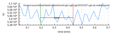
When using the single TIC intensity value function, any feature of a plot will be integrated to a single TIC value that represents the sum of all the TIC values for all the MS data in the MS run data set that match the feature selection. The obtained single TIC intensity value is displayed at the bottom of the plot widget in which the calculation was requested. In this example, the feature that was selected for integration is located between the vertical markers.
Figure 2.13: Single TIC intensity value for any mass spectral data feature #
 This is the check button that, when
pressed, directs the new integration to produce a
int = f(m/z,rt) color map. This function is only useful for
mass spectrometric data sets that were acquired in
“profile” mode; that is, for acquisitions performed along a
time frame, like an on-line chromatography-MS experiment.
This is the check button that, when
pressed, directs the new integration to produce a
int = f(m/z,rt) color map. This function is only useful for
mass spectrometric data sets that were acquired in
“profile” mode; that is, for acquisitions performed along a
time frame, like an on-line chromatography-MS experiment.
 This is the check button that, when
pressed, directs the new integration to produce a
int = f(m/z,dt) color map. This function is only useful when
the mass spectra were acquired during an ion mobility mass spectrometry
experiment.
This is the check button that, when
pressed, directs the new integration to produce a
int = f(m/z,dt) color map. This function is only useful when
the mass spectra were acquired during an ion mobility mass spectrometry
experiment.
 This is the check button that, when
pressed, directs the new integration to produce a
int = f(dt,rt) color map. This function is only useful for
mass spectrometric data sets that were acquired in an ion mobility mass
spectrometry experiment.
This is the check button that, when
pressed, directs the new integration to produce a
int = f(dt,rt) color map. This function is only useful for
mass spectrometric data sets that were acquired in an ion mobility mass
spectrometry experiment.
2.7.3 The Plot Widget Main Menu #
There are two kinds of plots: the trace plots, like mass spectra, drift spectra, TIC chromatograms, and the color map plots, like the int = f(dt, m/z) color map, for example. In the two cases, the menu is not the same because the features of the plots are not the same.
2.7.3.1 The Trace Plot Widget Main Menu #
The trace plot widgets can host any number of traces, be them drift or mass spectra or TIC chromatograms. A trace is a curve-type graph, that is, a two-dimensional graph. The intensity is at the Y axis and the X axis hold either m/z, dt or rt values. The trace plots all share the same main plot widget menu.
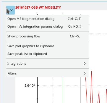
The main menu provides actions that may apply only to the plot widget that owns the menu.
Figure 2.14: Trace plot widget main menu #
Tip
The menu items described below perform actions that apply to individual plots inside the plot widget that owns the menu. mineXpert2 tries to understand the will of the user: when only one plot is in the widget, the menu action applies to that plot, even if it is not currently selected. As soon as there are more than one plot in the widget, the action requires that the target plot be selected. If no plot is selected, a dialog window will instruct the user to select the specific plot of interest.
: Open a dialog to set the MSn requirements for the MS data integration (see Section 3.1.2, “Setting the MSn fragmentation parameters”).
: Open a dialog to set the m/z integration parameters (see Section 3.1.3, “Setting the m/z integration parameters”).
: Open a dialog and display the processing flow of the currently selected graph. If there is only one graph in the plot widget, the processing flow for that graph (even if it is not selected) is shown.
: Save the whole plot widget as a graphics object to the clipboard.
: Save the currently selected (or unique) trace to the clipboard as numerical data.
→ : integrate the data by moving the cursor over each point of the current trace. Click on the starting trace at the place where point-by-point integration needs to start, then use the F3 to integrate the next plot point.
→ : the filter will be run with the configuration settings configured as at Section 3.1.6, “Savitzky-Golay filtering of any kind of data”. The smoothed trace will be added into any pinned-down plot widget of the receiving window. If no plot widget is pinned-down, then a new plot widget will be created.
2.7.3.2 The Color Map Plot Widget Main Menu #
The color map plot widgets can host only one color map since it is not possible to overlay more color maps onto a color map. A color map is a raster-type graph, that is, a bitmap image of which the third dimension is the intensity of the pixel at any given position in the image. That intensity is represented as a color. The color map plots all share the same main plot widget menu that is significantly different than the menu available in trace plot widgets.
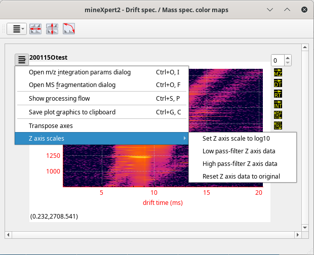
The main menu provides actions that may apply only to the plot widget that owns the menu.
Figure 2.15: Color map plot widget main menu #
: Recompute all the intensities by calculating the new intensity as the log10 of the original intensity.
When the log10 scale is applied to the intensities of the previous color map plot, where almost no signal was visible, then the signal is made perfectly visible."
The switch to a log10 scale for the intensities might reveal a lot of missing signal when the intensities are used in a linear scale. The drawback is that noise can be hugely enhanced. See below for a way to reduce that noise.
Figure 2.16: Color map plot widget main menu #
: The value that is entered in the input box that is shown is a percentage of the maximum intensity over the whole map. The function first computes a threshold using the formula threshold = percentage * max_int / 100. All the cells having an intensity value above that threshold have their value set to that threshold value. All other cells are unchanged. This function is used to reduce the dynamic range of the map and potentially enhance features of interest.
: The value that is entered in the input box that is shown is a percentage of the maximum intensity over the whole map. The function first computes a threshold using the formula threshold = percentage * max_int / 100. All the cells having an intensity value below that threshold have their value set to that threshold value. All other cells are unchanged. This function is typically used for removing noise.
2.8 General Operation of the Plot Widgets #
All the plot widget-containing windows, like the TIC/XIC chromatograms, Mass spectra and Drift spectra windows, all contain plot widgets that have a general working scheme as to how the data can be visualized. The main visualization operations are succintly described below. The following convention will be used to describe the mouse buttons:
 : left mouse button;
 : middle mouse button;
 : right mouse button.
Note
All the visualization operations are performed using the
left mouse mutton (). Keyboard keys are used to
better qualify the zoom-in/-out or panning operations.
The different plot or colormap graph visualization methods are detailed below:
Zooming-in and zooming-out:
Zoom-in:
-click-drag to draw a selection rectangle.
When the mouse button is released, the new plot view contains the data
contained in the selection rectangle. Note that if the mouse drag over
the y-axis spans less than 10 % of the vertical scale, the
rectangle does not show up because the software thinks that the mouse
drag operation is only horizontal (which has a meaning described later).
Zoom-in: Ctrl+
-click-drag along the x-axis
over the region to zoom and release the mouse button. The new zoomed
view contains the mouse drag-spanned region. The y-axis spans the
region contained between the initial plot bottom y-value and the
position on the y-axis of the mouse during the drag operation.
The start and end x locations are visualized with green and red markers, respectively. The x-axis distance between the markers is refreshed all along the mouse movement.
Figure 2.17: Zooming-in operation #
Zoom-in/-out: Ctrl+
-click-drag
onto either the x- or the y-axis to
interactively zoom-in or -out along that selected axis. In this
mode, the zoom operates by contracting/expanding the data in such a
manner that the left/bottom part of the graph (the origin of the
graph) is anchored and does not move. When the drag occurs towards
larger values on the clicked axis, the view is zoomed-in along that
axis. Conversely, it is possible to zoom-out by dragging the mouse
towards lower axis values.
Zoom-in/-out: The
-wheel-rotation can be used to zoom-in or -out
the whole plot on both the x- and y-axis simultaneously. Note that the
position of the mouse cursor when the wheel is rolled defines the new view of
the plot. Practising a bit allows to make that zooming-in/-out mode very
powerful.
Zoom-out: To reset the zoom along one axis,
-double-click
that axis. In this case, only the clicked axis will be full-scale, the other
axis remains unchanged. To reset the zoom on both axes in one go,
-double-click one of the axes maintaining the Ctrl key
pressed;
Panning:
-click-drag on one of the axes to pan the plot view along
that axis; Relative full-scaling along the y-axis: in almost all of the zooming operations described above, it is possible to ensure that the y-axis is full-scaled automatically to the most intense peak visible in the zoomed region by pressing the Shift key.
Recording the history of zoomed views:
Each time a new zoomed-in/-out view of the plot is triggered, a history element is stored in the plot widget. To back-replay the various steps of the zoom-in/-out operations in sequence, from pre-last to first, hit the Backspace key. The exceptions to this mechanics is when the plot view is zoomed using the mouse wheel.
Note: Locking the x and y axes of all the plots
The tool bar located at the top of all the plot widget-containing windows described above contains two buttons that allow to lock the x-axis (the button icon has the horizontal red line) and the y-axis (red line is vertical) range throughout all the plot widgets in the window. This is of great use when the user wants to compare a number of graphs that have been obtained on comparable samples. The movements and zoom-in or zoom-out operations in one graph are then synchronized to all the other graphs.
[7] Please, see http://proteowizard.sourceforge.net/
[8] TIC stands for “total ion current” and XIC stands for “extracted ion current”.
[9] Combination of color maps is not yet implemented, although they might be useful in some situations.